Adaptive Layer Slicing for Variable-Diameter 3D Printing: Algorithm, Benchmarks, and Trade-offs
By Jacob Cossette
A special project done for Aptus Tech, a Centech-incubated startup, to solve a slicing problem no existing software could handle: preparing 3D models for a print head with a variable nozzle diameter.
The problem
Aptus Tech was developing a 3D printer with a variable-diameter print head, hardware capable of switching nozzle diameter mid-print to trade off speed against precision within a single object. The hardware side of that idea is only half the problem. Every slicer on the market assumes a fixed nozzle diameter, so none of them can generate a toolpath that varies resolution locally, printing coarse layers where precision doesn't matter and fine layers exactly where it does. That gap is what this project set out to close: a proof-of-concept slicing algorithm for variable-diameter printing, plus a functional prototype to measure whether the idea actually pays off.
The core technical idea: cusp height as the error signal
The algorithm needs a way to decide, for any given region of a model, whether the current layer thickness is good enough or needs refining. The metric used for that is cusp height, a standard concept in adaptive slicing research (Mani et al., 1998): the deviation between a printed layer's surface and the ideal surface of the 3D model, given by
h = r · (1 − cos(θ/2))
where r is the local radius of curvature of the surface and θ is the angle between two adjacent contour points. A high cusp height means the surface is curving quickly relative to the current layer thickness, which is exactly where visible ridges and inaccuracies appear.
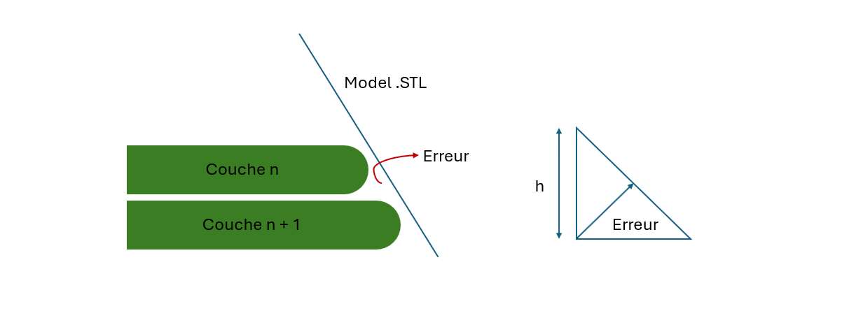
Cusp height, visualized: the gap between a flat printed layer and the model's sloped surface (left) is the error the algorithm measures and reduces to a simple triangle (right) to compute h.
The pipeline built around this metric works in stages: import the STL file (a set of triangles, each defined by three vertices and a normal), compute the intersection between each triangle and a horizontal cutting plane using linear interpolation to build the contour polygon for that layer, then evaluate cusp height along that contour to flag regions where the error exceeds a defined tolerance. In flagged regions, the algorithm inserts sub-perimeters, essentially finer internal layers nested inside the coarse one, sized so their combined thickness still equals a clean multiple of the base nozzle diameter (so a 0.3 mm target can be reached as two 0.1 mm sub-layers without misalignment between layers).
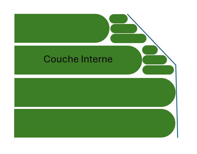
Where the error is flagged, the algorithm nests finer sub-perimeters inside the coarse layer rather than refining the whole object — resolution goes up locally, not globally.
Choosing what to build versus what to reuse
Three approaches were evaluated before settling on the final architecture, and it's worth being explicit about why each earlier option was dropped:
OpenGL, for a custom STL viewer and rendering pipeline. This gave full control but ran into a hardware compatibility wall (a GLFW/WGL driver error on the available GPU) and, more importantly, building a performant STL viewer from scratch (large file handling, rotation, translation) turned out to be a much bigger scope than the slicing algorithm itself. Dropped for scope reasons.
Assimp, an established library for importing 3D formats with useful geometry utilities (triangulation, vertex extraction, normal handling). It solved the import problem well but still required building the entire toolpath generation logic from nothing. Kept in mind as a strong option for a future, full slicer rewrite, but too incomplete for the timeline of this project.
Slic3r, a mature open-source slicer with toolpath generation already built in. Using it would have meant working inside an architecture with limited control over the internals, exactly the layer the algorithm needed to modify.
The approach that actually shipped: taking a much simpler, already functional open-source Python slicer (originally by Aaron Schaer and Michelle Ross) and extending its Slice object with new sub-perimeter attributes, rather than building a slicer from zero. That decision (reuse a small, understandable codebase and add exactly the one capability needed) is what made it possible to get to measurable results within the project timeline.
Benchmark methodology: isolating the effect of the algorithm, not the printer
To know whether adaptive slicing was actually worth it, the comparison had to control for everything except the slicing strategy. Three geometries (a cube, a sphere, and a ring, chosen to range from flat surfaces to continuous curvature to combined convex/concave curvature) were sliced three ways: constant 0.5 mm diameter, constant 1.0 mm diameter, and the adaptive algorithm. All other print parameters were held fixed across every run: 50% infill, filament cost of $0.08/gram, 15 mm/s extrusion speed, 45 mm/s travel speed. For each of the nine resulting prints, five metrics were captured: print time, number of layers, object mass, filament length used, and print cost.
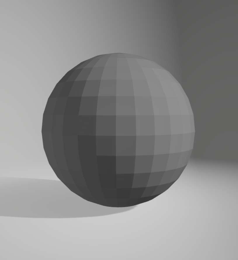
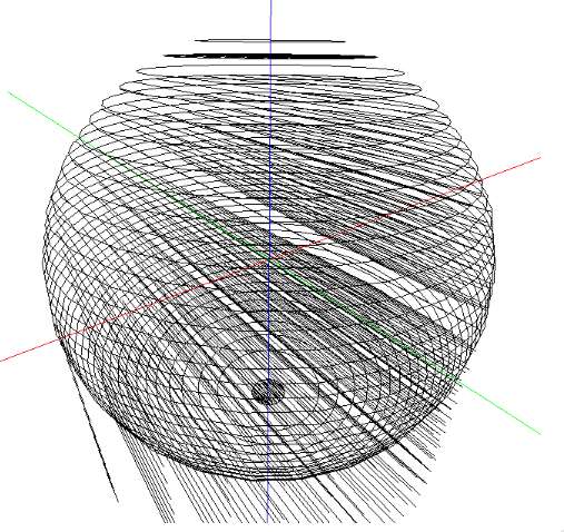
One of the three test geometries: the source sphere STL (top) and the adaptive algorithm's generated toolpath (bottom) — continuous curvature everywhere is exactly the case where variable resolution has the most to offer.
Results: a quantified speed/precision trade-off
The adaptive algorithm consistently landed between the two constant-diameter baselines, which is the expected result, but the interesting part is by how much. Averaged across the three test geometries, moving from a constant 1.0 mm diameter to the fully adaptive algorithm increased print time by only 18.54%, while achieving the surface precision of a constant 0.5 mm print, which itself requires a 147.7% increase in print time over the 1.0 mm baseline. In other words, the adaptive approach captured most of the precision gain for roughly an eighth of the time cost. It also used the same base layer count as the coarse 1.0 mm print (20 layers instead of 40 for the cube, 10 instead of 20 for the ring), refining resolution only in the flagged regions rather than doubling every layer across the whole object.
The gap between geometries was also informative: the time cost of the finer sub-perimeter logic scaled with curvature complexity, from a cube (mostly flat faces, least benefit from adaptive resolution) to a ring (continuous curvature everywhere, largest relative gain). That's a useful signal for where this technique matters most in practice: highly curved or organic geometries, not simple prismatic shapes.
What still doesn't work, and why that's worth publishing
The proof of concept reached its core goal, quantifying whether variable-diameter slicing is worth building, but three concrete limitations remain unresolved, and each has a clear next step:
Perimeter/infill overlap. Depending on which perimeter reference the infill algorithm uses, prints either leave a gap between the outer wall and the internal fill (weakening the part structurally) or the infill overlaps the sub-perimeter (risking print errors). The likely fix is defining each perimeter and sub-perimeter with its own explicit thickness rather than treating them as zero-width reference lines.
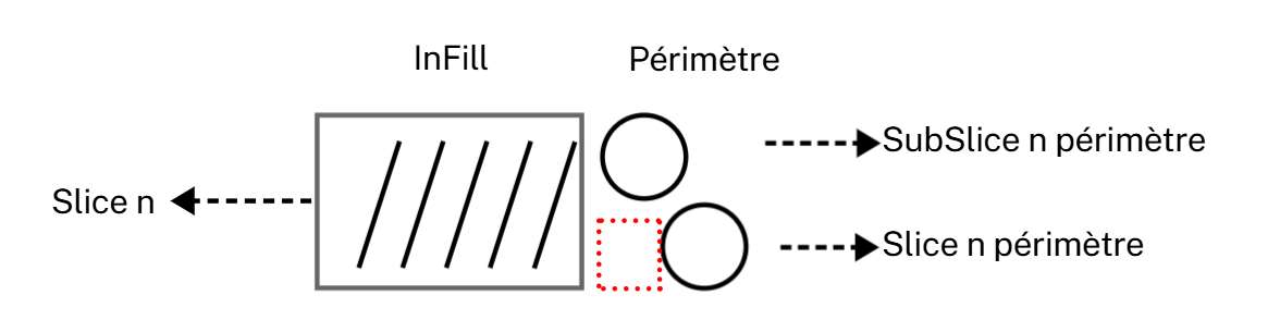
One failure mode of the current perimeter reference: a gap opens up between the outer wall and the internal infill (highlighted), weakening the part. The report also documents the opposite failure — infill overlapping the sub-perimeter.
Processing time. Generating G-code for the cube took 32 seconds on an Intel Core i7-6600U; the sphere took 103 seconds; the ring took 1,457 seconds. That curve (roughly 45x slower for a moderately more complex shape) is a Python-implementation ceiling more than an algorithmic one, and the report's own recommendation is a rewrite of the hot path in C++.
Toolpath optimization. The current implementation doesn't minimize travel moves between segments, producing visibly redundant back-and-forth motion on both the sphere and cube test prints. This doesn't affect precision but does affect real print time and wear, and it's a known, tractable class of problem (travel-path optimization) that simply wasn't in scope yet.
Takeaways
Evaluate the build-versus-reuse decision explicitly, and document why each rejected option was rejected. That record is what let this project land on the right-sized solution instead of re-deriving it by trial and error. Design benchmarks as controlled comparisons, not single demos: fixing every variable except the one under test is what turned "the adaptive algorithm seems better" into a specific, defensible number (18.54% versus 147.7%). And report limitations with the same rigor as results. A proof of concept that states exactly what still breaks, and why, is more useful to the next engineer (or investor, or customer) than one that only shows the wins.
Download the full report (PDF): full technique review, cusp-height derivation, benchmark tables, limitation diagrams, and installation instructions for the slicing prototype.